
Phonons from a universal potential: the PET-MAD cookbook recipe
I spend most of my time computing phonons the orthodox way — finite displacements or DFPT on top of a periodic hybrid-DFT calculation, with all the attendant bookkeeping: acoustic sum rule, Born charges and LO–TO splitting, supercell convergence, and occasional spurious imaginary modes that turns out to be artifacts rather than real instabilities. So when I went looking through The Atomistic Cookbook to get inside the COSMO software stack, the recipe Phonon dispersions with unconstrained models and uncertainty quantification (Paolo Pegolo and Michele Ceriotti) was the obvious place to start: familiar ground, computed with tools I had not used before.
This is my reading of that recipe in the spirit of a phonons person exploring new territory.
What the recipe computes
The construction is the standard frozen-phonon one, with a single substitution: the forces on displaced supercells come from a machine-learning interatomic potential — PET-MAD, a universal potential built on the Point Edge Transformer architecture and trained across 102 elements at the r2SCAN level — rather than from DFT. In the harmonic approximation the dynamical matrix at wavevector \(\mathbf{q}\) is
\[D_{\alpha\beta}(\kappa\kappa';\mathbf{q}) = \frac{1}{\sqrt{m_\kappa m_{\kappa'}}} \sum_{l'} \Phi_{\alpha\beta}(0\kappa; l'\kappa')\, e^{\,i\mathbf{q}\cdot[\mathbf{r}(l'\kappa') - \mathbf{r}(0\kappa)]},\]with the real-space force constants \(\Phi\) obtained from finite differences of
the MLIP forces. Negative eigenvalues are reported
as imaginary (plotted as negative) frequencies and flag a dynamical
instability: the structure is a saddle point of the potential-energy surface,
and some distortion lowers the
energy. Two features lift this above a routine phonopy run. The model is
unconstrained (PET does not enforce crystal symmetry or exact rotational
equivariance; symmetry is recovered only approximately), and the bands carry
uncertainty estimates from a shallow ensemble, with committee members built
through the last-layer prediction rigidity framework. The ensemble machinery is
uqphonon, a wrapper around
phonopy and
i-PI.
Three systems carry the tutorial: FCC aluminium (a stable metal), rhombohedral \(R3m\) BaTiO\(_3\) (the ferroelectric ground state), and cubic \(Pm\bar{3}m\) BaTiO\(_3\) (the paraelectric structure, dynamically unstable).
The unconstrained-symmetry pitfall
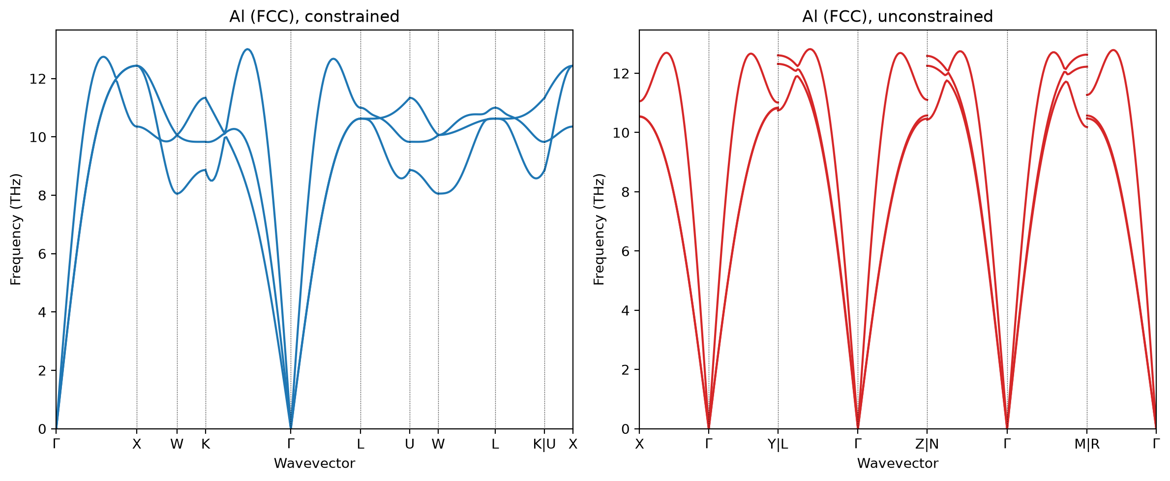
The aluminium example is built around a subtlety that conventional DFT hides
from you. Relax FCC Al without a symmetry constraint and the model’s residual
non-equivariance acts as a small (\(\lesssim 10^{-3}\)) symmetry-breaking field;
the optimizer follows it into a cell that spglib reads as \(Fm\bar{3}m\) at loose
tolerance but \(P\bar{1}\) at tight tolerance. The automatic \(\mathbf{q}\)-path
finder then picks a generic triclinic path, and the dispersion looks different
from the constrained one — even though the underlying force constants are
essentially identical.
Put both on the same explicit FCC path and the point is made: the constrained and unconstrained dispersions overlap almost perfectly, the small residual differences being the numerical symmetry-breaking itself.
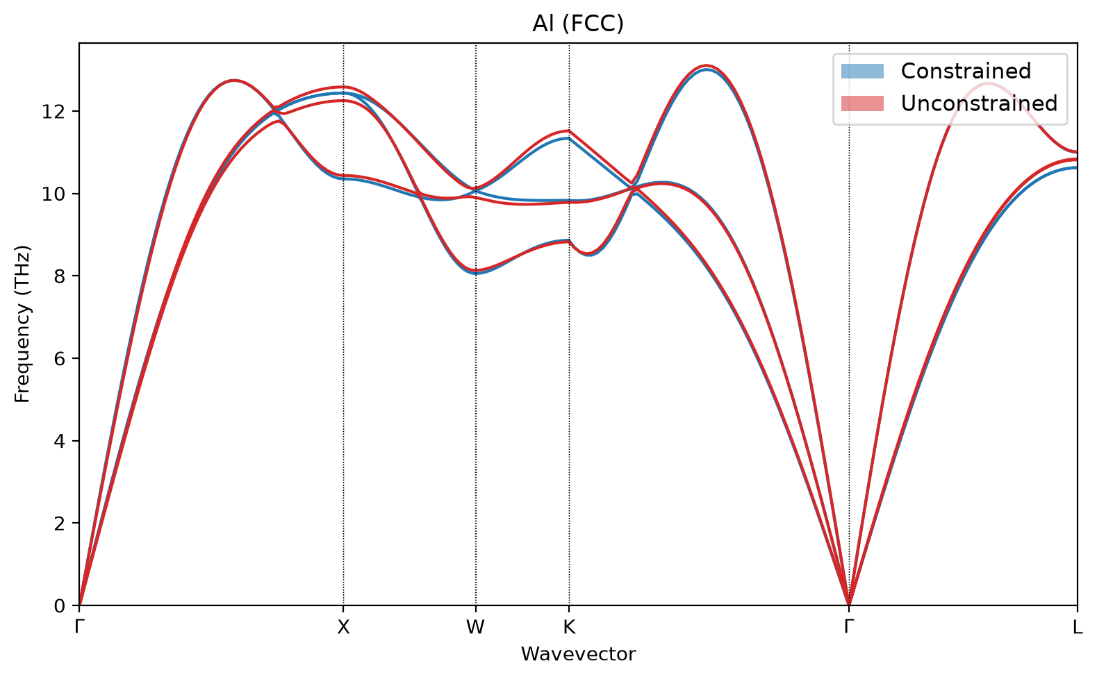
Because unconstrained models lack inherent structural constraints, enforcing a rigorous protocol is mandatory. In practice, you must either apply FixSymmetry during the relaxation process or use spglib.standardize_cell to restore exact symmetry prior to phonon calculations.
Uncertainty bands
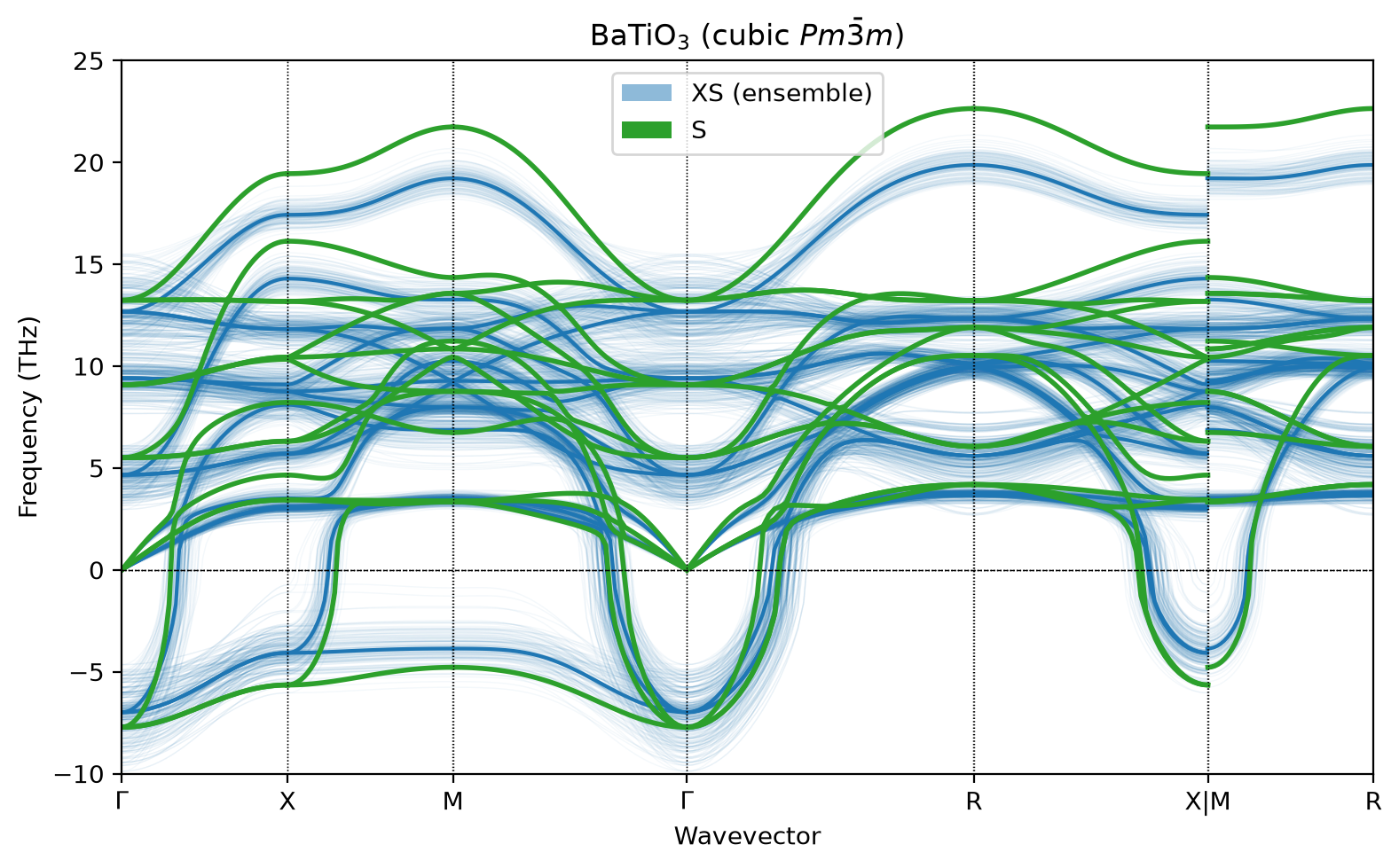
The uncertainty quantification is the other half of the recipe. Each committee member yields its own force constants, hence its own dispersion; the band is drawn as the ensemble mean with a \(\pm\sigma\) shading. Comparing the XS model’s ensemble against the larger S model is the recipe’s self-consistency check.
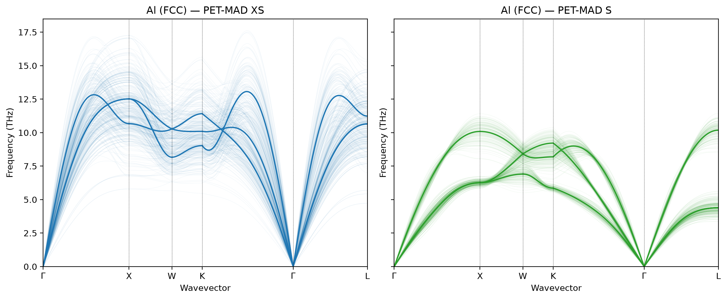
A caveat worth stating plainly: these bands estimate epistemic model uncertainty propagated through the harmonic problem. They do not include the systematic error of the r2SCAN reference the model was trained on, finite-supercell truncation of the force-constant range, or the finite-displacement anharmonic bias.
BaTiO\(_3\): a stable ground state and an unstable sheet
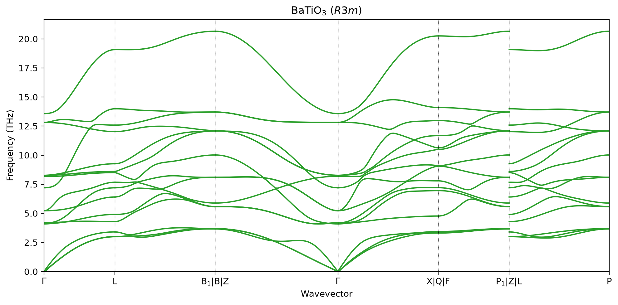
The rhombohedral \(R3m\) phase — the ground state discovered by unconstrained relaxation — comes out all-real, confirming dynamical stability.
The cubic \(Pm\bar{3}m\) phase is where it gets interesting, and where the full Brillouin-zone path earns its keep. The instability is not a zone-centre point. Along Γ–X–M the lowest branch stays imaginary and remarkably flat (≈ −4 to −7 THz), and it remains unstable through the X|M–R region, while it hardens toward R along ⟨111⟩ (Γ–R). That flat unstable manifold perpendicular to the ⟨100⟩ axes is the textbook signature of BaTiO\(_3\)’s chain-correlated, mixed displacive–order/disorder character (Comès; Yu–Krakauer; Zhong–Vanderbilt): Ti displacements are strongly correlated along ⟨100⟩ chains and weakly coupled between them. The genuinely notable result is that a universal MLIP reproduces the entire unstable sheet, not merely the \(\Gamma\) soft mode.
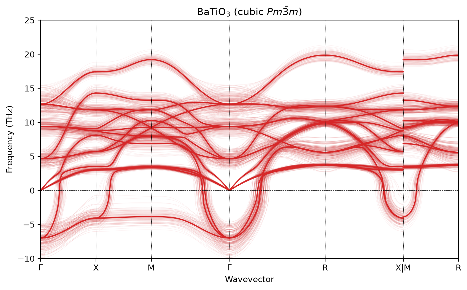
| Cubic BaTiO3 (PET-MAD XS ensemble). The triply-degenerate ferroelectric soft mode reaches ≈ −7 THz at Γ, but the instability extends as a flat sheet along Γ–X–M and through X | M–R — the hallmark of the chain-correlated transition. |
Overlaying the S model on the XS ensemble shows the two agree on the instability structure and on the ≈ −7 THz \(\Gamma\) depth, while diverging on the high optical branches (S pushes the top mode to ~22 THz against ~20 THz for the XS mean). The ensemble spread is large precisely where the models disagree — the high optical manifold — and tight on the acoustic and soft branches.
Reading it as a phonons person
The recipe is a good and fast tutorial. However, some pieces of lattice-dynamics physics sit outside its scope:
No non-analytical correction, hence no LO–TO splitting. Both BaTiO\(_3\)
phases are polar insulators, yet no Born effective charges \(Z^{*}\) or
high-frequency dielectric tensor \(\varepsilon^{\infty}\) enter the workflow, so
the LO–TO splitting at \(\Gamma\) is absent from every BaTiO\(_3\) dispersion. This
is not a bug one can fix inside the model — an energy/force MLIP carries no
polarization information — but it is a real omission for a ferroelectric, where
the LO–TO splitting is central. The repair is to inject externally computed
\((Z^{*},\varepsilon^{\infty})\) from a separate DFPT or finite-field calculation
through phonopy’s nac_params.
Rotational invariance is not enforced. phonopy’s symmetrize_force_constants
imposes the translational acoustic sum rule, \(\sum_j \Phi_{\alpha\beta}(i,j)=0\),
and permutation symmetry — but not the Born–Huang rotational sum rules. For the
3D bulk crystals here that omission is negligible; for the layered and
two-dimensional systems I work on it is exactly what corrupts the quadratic
flexural (ZA) branch near \(\Gamma\), often as a spurious small imaginary pocket
that mimics an instability — a failure mode I ran into directly in
SnSe\(_2\). Reproducing this workflow for a monolayer would
require rotational-sum-rule enforcement
(hiPhive does this) on top of phonopy.
Takeaways
PET-MAD plus the standard phonopy machinery reproduces qualitative lattice
dynamics (including the extended ferroelectric instability) with
calibrated model-uncertainty bands, and the UPETCalculator-as-ASE-calculator
design means an existing DFT-based phonon workflow ports over by changing
essentially one line. A clean comparison of soft-mode frequencies across model families, with NAC wired in and a 2D test
case under rotational sum rules, is the natural next step.
Links
- Recipe: Phonon dispersions with unconstrained models and uncertainty quantification, P. Pegolo and M. Ceriotti (BSD-3-Clause)
upet(PET-MAD and friends): https://github.com/lab-cosmo/upetuqphonon: https://github.com/ppegolo/uqphononphonopy: A. Togo, J. Phys. Condens. Matter 35, 353001 (2023)- PET-MAD: A. Mazitov et al., Nat. Commun. 16, 10653 (2025)